Overview

1 Polar Axis

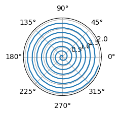
For a demonstration of a line plot on a polar axis, see Figure 1. Equation 2

Black-Scholes (Equation 1) is a mathematical model that seeks to explain the behavior of financial derivatives, most commonly options:

\frac{\partial \mathrm C}{ \partial \mathrm t } + \frac{1}{2}\sigma^{2} \mathrm S^{2} \frac{\partial^{2} \mathrm C}{\partial \mathrm C^2} + \mathrm r \mathrm S \frac{\partial \mathrm C}{\partial \mathrm S}\ = \mathrm r \mathrm C \tag{1}

\mathcal{M}

\mathcal{L} \tag{2}

(Wikipedia 2022) Equation 2 ?@eq-stddev1

Code

i = 3

Code

i + 7

Code

import numpy as np
import matplotlib.pyplot as plt

for i in range(2):
    r = np.arange(0, 2, 0.01)
    theta = 8 * np.pi * r
    fig, ax = plt.subplots(
      subplot_kw = {'projection': 'polar'} 
    )
    fig.set_size_inches(2,2)

    ax.plot(theta, r)
    ax.set_rticks([0.5, 1, 1.5, 2])
    ax.grid(True)
    plt.show()

(a) Gapminder: 1957

(b) Gapminder: 2007

Figure 1: Life Expectancy and GDP

Code

from math import pi
from random import uniform

from ipywidgets import Button

from ipycanvas import Canvas, hold_canvas


     

canvas = Canvas(width=300, height=300)


     

def recursive_draw_leaf(canvas, length, r_angle, r_factor, l_angle, l_factor):
    canvas.stroke_line(0, 0, 0, -length)
    canvas.translate(0, -length)

    if length > 5:
        canvas.save()

        canvas.rotate(r_angle)
        recursive_draw_leaf(
            canvas, length * r_factor, r_angle, r_factor, l_angle, l_factor
        )

        canvas.restore()

        canvas.save()

        canvas.rotate(l_angle)
        recursive_draw_leaf(
            canvas, length * l_factor, r_angle, r_factor, l_angle, l_factor
        )

        canvas.restore()


     

def draw_tree(canvas):
    with hold_canvas():
        canvas.save()

        canvas.clear()

        canvas.translate(canvas.width / 2.0, canvas.height)

        canvas.stroke_style = "black"

        r_factor = uniform(0.6, 0.8)
        l_factor = uniform(0.6, 0.8)

        r_angle = uniform(pi / 10.0, pi / 5.0)
        l_angle = uniform(-pi / 5.0, -pi / 10.0)

        recursive_draw_leaf(canvas, 150, r_angle, r_factor, l_angle, l_factor)

        canvas.restore()


     

button = Button(description="Generate tree!")


def click_callback(*args, **kwargs):
    global canvas

    draw_tree(canvas)


button.on_click(click_callback)


     

draw_tree(canvas)


     

display(canvas)
display(button)

Code

from ipyleaflet import Map, Marker, basemaps, basemap_to_tiles
m = Map(
  basemap=basemap_to_tiles(
    basemaps.NASAGIBS.ModisTerraTrueColorCR, "2017-04-08"
  ),
  center=(47.26327165045244, 11.400229023615665),
  zoom=4
)
m.add_layer(Marker(location=(47.26327165045244, 11.400229023615665)))
m

References

Wikipedia. 2022. “Absorptionskoeffizient — Wikipedia, the Free Encyclopedia.” http://de.wikipedia.org/w/index.php?title=Absorptionskoeffizient&oldid=208046932.